Etch Your Own Circuit Boards

Etch Your Own Circuit Board

                                                                                By Bill Johnson KI4ZMV

Does this look familiar? This was an earlier project.  It consists of a +/- 5-volt power supply driving an op-amp, which in turn turns on and off a clock, whenever the attached HT senses a signal on our repeater. Nightmare wiring jobs like this make you wonder if there might be a better way.  There is. Etch your own circuit board.

Figure 1. This is hardly a model of neatness. A custom circuit board would have made this both neater and more reliable.

If the complexity of etching your own frightens you, have heart. It is not as difficult as you might think. You may be pleasantly surprised to learn that the necessary software is available free, and that the etching chemicals can be found at any Wal-Mart. Just follow these simple nine steps.

Step 1. Prototype The Circuit

Before we get to the chemistry, you will first need a working circuit. This in turn has to be turned into a piece of artwork, which will later be transferred onto a copper clad board. Figure 2 is a sketch of my prototype. This circuit converts RS232 to TTL using a Max232 chip. The board also contains a 5-volt voltage regulator. I built a breadboard version to verify that the circuit performed as expected from the sketch below.

Figure 2. This is the circuit from which the prototype breadboard was wired, with the exception of the regulator that was added later. Figures 17 and 18 below show the transition from breadboard to circuit board.

Step 2. Create The Artwork

Guided by the circuit sketch, in figure 2, the next step is to create the artwork needed to etch your board.

Figure 3. Artwork created using Express PCB 

There are many options for turning your circuit into artwork, but the one I prefer is the software provided by Express PCB. You will find their free software at: http://www.expresspcb.com/expresspcb/. After you’ve made a few boards yourself, you may want to have the pros make your next one. That’s up to you. The good news is that what you learn using their software will help you either way.

I will not go into using the software. The site above has excellent tutorials for that. I will assume you can get to the print stage.  Figure 3 is an example of the printed output.
Here is something to keep in mind. For this procedure, you will lay your board out as if the traces were on the top, even though when you are finished, they will end up on the bottom side of the board, with your components on top. In the transfer process, the image will be reversed if viewed from the rear, but correct if viewed through the board, from the top.

Step 3. Print The Artwork

To transfer your artwork to a copper clad board you will need to first print it using a laser printer, the kind that uses toner. Inkjet will not work! Set your printer for high quality, heavy lay down.

The paper you use is critical. You want a paper that has a clay coating. You can find this in any stationary store. It has a glossy, magazine page look. I got excellent results with HP Presentation Paper 120g. A 250-sheet pack will last you a lifetime.

Of course, you will need some copper clad board. You can purchase new, or look for a supplier that sells scraps.

Step 4. Prepare The Board

The surface of the board must be cleaned. Any grease on the board will interfere the etching process, and possibly prevent a good transfer from your paper image to the surface of the copper. I have used S.O.S Pads, and sometimes cleanser and a sponge. The important thing is to end up with clean, shinn copper. The two boards in the back are finished. The one in the front is being cleaned.

Figure 4. Cleanser is a good choice for cleaning the copper on the board.

Figure 5. You can tell the surface is clean when water does not bead, and the surface is bright and shinny. Notice how the water beads on the left side of this board, but sheets on the right.

Step 5. Transfer The Image

The clean dry board is placed on a flat work surface. I use a piece of scrap plywood to protect the kitchen counters. It is a good idea to use some double-sided tape on the back of the board to keep it from moving around during the transfer process.

With the board in place you are ready to transfer your printed image. Carefully lay the printed circuit image face down on the copper side of the board, and then tape it to your work surface. You don’t want it to move while you are applying heat and pressure.

Figure 6. The board is affixed to the work surface and under the sheet of paper containing the circuit. The image is face down.

The laser image consists of a heat sensitive resin. Our goal here is to re-melt this resin, and transfer it to the copper foil. Set the iron on high heat, and apply pressure. You will also want to move the iron around. Be careful not to move the paper. If you are concerned about the iron sticking you can place a sheet of standard copier paper over the one containing the image.

Step 6. Removing The Paper

Warning, the board will be hot after the transfer. Let it cool to the touch before you place it into a dish of warm tap water. Once in there, let it soak for a minute or so, gently rocking the dish back and forth.

After a time, the paper will become wet, and at that point you can gently peel it from the board. It will not all come off at once. Be patient.

Figure 7. After a minute or so the paper will come away from the board.

Figure 8. Most of the paper has been removed. Scrubbing with your fingers under running water will remove the rest.

At this stage you will have to gently scrub with your fingers to remove the last of the paper fibers. Don’t worry about damaging the transferred image. If everything went well up to this point, the toner has become one with the copper board.

Figure 9. This board is clean enough and ready for etching. Note, there are some imperfections, but nothing major.

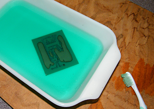
Step 7. Etch The Board

We are ready to etch away all the unprotected copper. You will need a mixture of two chemicals for this. Both can be found at Wal-Mart. The first chemical is hydrogen peroxide, the second is Muriatic acid.  Hydrogen peroxide can be found in the drug department. You will find Muriatic in the paint department. It is used for cleaning bricks. It is also used to adjust the ph of swimming pools.

A word of caution! Muriatic acid can be dangerous if mishandled. Follow these simple precautions. Always add water, or in this case peroxide, to acid, never the other way round. And most important of all, wear some kind of eye protection. I also like to be near a source of running water just in case. I know all this may sound a bit scary, but if you use some common sense and are careful, you will be fine. 

Figure 10. Notice I have a plastic measuring cup, and a glass tray for processing. Do not use aluminum, or other metal pan for etching. Use only glass or plastic.

The ratio of peroxide to acid is 2 to 1. For my board I measured out 4 ounces of acid, to which I added 8 ounces of peroxide making a total of 12 ounces. This was transferred to the glass baking-dish. Next I slid the board into the solution face up.

Figure 11. Board first immersed into the etching solution

Shortly after immersion, you will notice a dark discoloration form on the surface of the board. The chemicals are doing their job, but you have to help by gently rocking the tray back and forth. Alternately you can move the board around with an old toothbrush. Gently scrubbing the surface with the brush also helps. Be patient. The etching process takes about 30 minutes at room temperature. Rocking and scrubbing brings fresh chemical in contact with the copper, and at the same time moves the exhausted chemical out of the way.

Eventually all the copper will be eaten away leaving only the circuit traces.

Figure 12. Almost there.  Only  a couple islands of excess copper remain.

Step 8. Clean Resin From The Board

After all the exposed copper has been etched away, you will have to remove the toner from the board. This is done with some steel wool, or an SOS soap pad. You will be amazed at how well the resin stuck to your copper board at this stage. A good deal of scrubbing is required to remove it.

Figure 13. Steel wool is used to remove the resin from the image the remaining copper.

Figure 14 is what you are aiming for at this stage. All the unprotected copper has been removed, along with the resist. The foil is bright, shiny and ready for drilling.

Figure 14. The cleaned board, ready for drilling. Not perfect, but serviceable.

Step 9. Drilling

We are going to need some very small drills for this step. I bought a couple sets of these at Harbor Freight. They were inexpensive, and work quite well. You do have to be careful not to snap them. They are quite small. We will be using one with a diameter of 0.025 inches.

Figure 15. Drill sets purchased at Harbor Freight.

I’ve been told that you can do this by hand, but I think a drill press is the way to go, along with a lot of light and a set of powerful magnifiers.

Figure 16. Board drilling setup

Figure 17 shows is the finished board etched, drilled, and ready for components. You are viewing the traces through the translucent board lit from behind. The sixteen-pin socket dropped in nicely. The 0.025 holes gave just enough wiggle room to accommodate the 0.020 pins.

Figure 17.  Image of the finished board viewed with transmitted light. The foil pattern is on the bottom side.

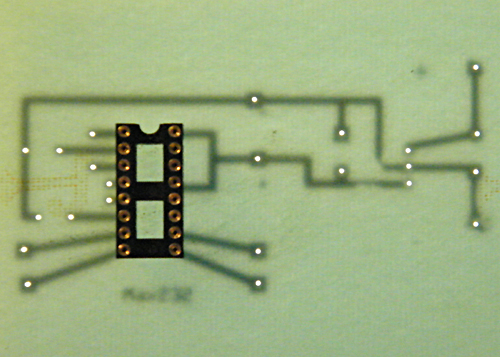
Here is the comparison of the finished circuit next to the breadboard version.

Figure 18. Breadboard next to final circuit board’s foil side.

Figure 19. Breadboard next to final circuit board’s topside. All components are in place with the exception of the Max 232 chip.

So here is a summary of the entire process:
1. Prototype the circuit
2. Create the artwork
3. Print the artwork on a laser printer using clay stock paper
4. Clean a copper clad board cut to size
5. Transfer the artwork to the board by applying heat
6. Remove the paper backing
7. Etch the unprotected Copper
8. Drill the holes
9. Populate the board

Not every project justifies your making a circuit board. They are a lot of work for something that will be used once or twice, and then placed on a shelf to collect dust. However, if your project will get some use, and more importantly, some day to day abuse, the circuit board is the way to go. The decision is yours. You now have the tools to fabricate your own circuit boards.

 

Measuring The Speed Of Sound With An Arduino And A $3 Sensor

Faster than a speeding bullet, able to bounce off walls in a single bound!

   Look! Over by the Arduino.

      It’s Super sound!                                                      by Bill Johnson, KI4ZMV

So you got your first Arduino program working. Great, you now have a thirty-dollar blinking light. How impressive is that? Not very. Perhaps the best ways to show off the power of the Arduino micro controller is to have it do something awesome. Measuring the speed of sound fits that description.

The Project

You can measure the speed of sound using the same principles found in digital tape measures. The difference will be that you fix the distance to a reflecting surface, and measure the time it takes for sound to make the round trip from sender back to receiver. From this you can calculate its speed using the formula:

speed =Distance/time

The Device

The device that makes this all possible is the HCSRO4 transmitter/receiver. I found this one on eBay. Look around. Prices vary. I paid about three dollars.

 

 Figure 1. The sensor is relatively small. The left side labeled T is the transmitter; the right, labeled R, is the receiver.

These units have only four connections: ground, echo, trigger, and Vcc. The left side marked T transmits a ping, while the right side labeled R listens for its return. The total distance traveled from the transmitter to a reflecting object and back, divided by the time it takes to make the round trip, is the speed of sound.

Wiring is straightforward.  There are only four connections. Connect sensor ground to Arduino ground, Vcc to Arduino five volts, the Trig pin to Arduino pin 13, and the echo pin to Arduino pin ll. Other combinations are possible. How simple is that?

Figure 2. The illustration above from www.toptechboy.com. A slightly modified   version of the program, appearing below, also came from this site.

The Test Setup

This is what my six-inch setup looked like. Yes, that is a napkin holder and a box of stick matches. Most likely your setup will be different.  

Figure 3 This is the six inch setup. The two probes connect the trig and echo pins to a scope. More below.

To make a reading, the trigger pin is brought LOW with a digital write. A pause follows to let things settle. After the pause the trigger pin is first brought HIGH then LOW again in quick succession. This LOW HIGH LOW sequence initiates, after a fixed delay, a ping and the start of the timing cycle. The ping will travel outward, bounce off a target, and then return, where it is registered by the echo pin. As soon as the echo is received, the timer stops, and the total time is set into the sketch variable called pingTime. PingTime, or travel time is measured in microseconds. Fortunately, the Arduino has a built in pulseIn(pin,state) library command that can be used to accurately measure pulse length.  

To get a better picture of what is happening, look at the dual trace scope output below from my Rigol Oscilloscope. Trace 1 shows the short initializing pulse, (upper trace), while trace 2 shows the resultant ping travel time (lower trace).

Figure 4. The scope’s scale is 500-microseconds per division horizontal, and 5 volts per division vertical.

The short pulse on trace1 was 10-microseconds long. The delay between this start pulse and the beginning of the timing pulse was 460 microseconds. This time is fixed, and independent of both the length of the initial short pulse as well as the measured time. With a distance of six inches from the reflecting surface to the sensors, the travel time was around 870-microseconds at room temperature.

The Arduino Sketch

Start by setting some variables. First, we need variables to identify the trig pin and echo pin. These will be type int. We also need three additional variables, one to represent ping travel time, another to represent the calculated speed of sound, and a third to represent the distance to the target. These will be type float.

In setup we initialize the serial monitor. This will be used for output. This is also the place we set the pin mode for the trig and echo pins.

In loop we bring the trig pin low, wait two seconds, then bring it high for 10 microseconds, then low again. This initializes the pulse read process. (More below.) Next we set the ping time equal to the pulse length reported by the Arduino pulseln function.

Calculation of the speed of sound is a matter of distance traveled divided by time. Distance is twice the target distance in inches, and time is the returned value of pulse length in microseconds. The inches per microsecond must then be scaled to miles per hour. Here is the completed sketch:

The Arduino Sketch

int trigPin = 13; //set trig pin to Arduino pin 13

int echoPin= 11; //set echo pin to Arduino pin ll

float pingTime;  //a variable to hold elapsed travel time to and from the target

float speedOfSound; //a variable to hold the speed of sound

float targetDistance=6; //a variable to hold the target distance. This will differ by test condition.

void setup() {

  Serial.begin (9600);  // start the serial monitor

  pinMode(trigPin,OUTPUT); //set the trigPin to OUTPUT

  pinMode(echoPin,INPUT); //set the echoPin to INPUT

}

void loop() {

  digitalWrite(trigPin, LOW);  //pull trig pin low

  delayMicroseconds(2000);  // delay to let things settle

  digitalWrite(trigPin,HIGH); //start initializing short pulse

  delayMicroseconds(10);  //pulse length

  digitalWrite(trigPin,LOW); //pull pulse low

  pingTime=pulseIn(echoPin,HIGH); //set pingTime to measured pulse length

  speedOfSound= 2*targetDistance/pingTime; //calculate speed of sound in inches per microsecond

  speedOfSound=speedOfSound *3600*1000000/63360; // convert to mph

  Serial.print("The speed of sound is "); //this line can be commented out for spreadsheet analysis

  Serial.print(speedOfSound); //print speed of sound

  Serial.println(" miles per hour"); //this line can be commented out for spreadsheet analysis

  delay (1000); //short delay for display purposes

}

Note, during testing I found it helpful to comment out the verbiage and print only values. This made transfer to a spreadsheet easier.

The Speed Of Sound And Ambient Temperature

The speed of sound varies with temperature. The following relationship is approximate, but accurate enough for our purposes. 

V=0.7341Tf +717.22

V is the speed of sound in mph

Tf  is the temperature in degrees Fahrenheit

From this we can generate a plot of the speed of sound in miles per hour versus temperature in degrees Fahrenheit, and a brief table to get a sense of the changes you might expect going from room temperature to either lower or higher temperatures.

Figure 5. Graphical and tabular results from the equation given above. These are the expected values for speed of sound at various temperatures.

From the graph and chart above we should expect the speed of sound to decrease at lower temperatures. Specifically, we would expect a 59 miles per hour decrease in the speed of sound going from an ambient temperature of 80F to 0F degrees.

To test this hypothesis, the apparatus was placed a refrigerator’s freezer section, whose temperature was zero degrees F. Though the data is noisy, it does suggest, that on the average, good agreement between the expected drop of 59 mph. The noise in the data cannot be accounted for at this time. One possible cause might be moisture buildup on the sensor.

  Figure 6. The drop in the speed of sound is obvious.

The Effect Of The Initial Pulse Length

Mentioned above was the apparent independence, within limits, of the initial pulse duration. Trigger pulse lengths of 10 to 200 microseconds were evaluated for their affect on the delay time between the end of the pulse and the start of the timing cycle. None was found.

Figure 7. The timing cycle, and the effect of initial pulse/trigger length

The Sensitivity Of Target Distance From the Sensor

The placement of the reflecting surface vis-a-vis the sensor is critical, especially at distances of around six inches. A series of measurements were made to determine the sensitivity of this parameter on the measured speed experimentally. Successive sheets of plywood were added to shorten the path. Each sheet was approximately 0.23 inches in thickness.

Figure 8. Testing the sensitivity to distance from the sensor at a nominal six inches.

Test results indicate the expected variation in apparent speed due to error in sensor to target distance. From the accompanying chart and its regression equation this is approximately 13.7 mph error for every increment of 0.1 inches. This is quite sensitive.

 

Figure 9. Sensitivity to distance from the sensor to reflector at nominal six inches.

It is assumed that placement of the sensor would be less sensitive if the distance were farther away. A test was run at thirty-six inches, and the results support the assumption.

Figure 10. This setup was used to measure the sensitivity of the sensor to target distance with a nominal distance of 36 inches.

Figure 11. Sensitivity to distance from the sensor to reflector at nominal thirty-six inches

From the chart,, regression equation, and table above it is clear that the sensitivity to distance from the target is much less. The regression equation suggests only about a 2.0 mph error for every 0.1 inches from nominal. We would expect that the sensitivity would be about six times as great for the nominal six inches versus the nominal thirty-six inch setups. Experimentally, the ratio was 6.9 ratio, or an error of approximately 15%.

Conclusion: We have demonstrated a practical way to measure the speed of sound using an inexpensive sensor and an Aduino. The sensitivity to ambient temperature and target distance were also explored.

A good friend of mine told me that if he ever needed to know the speed of sound he would Google it. This is a reasonable answer. You could also tell your grandson to Google it, or perhaps you could introduce him to the Arduino. How cool is that?

Session two- trouble shooting

Session two with the oscilloscope demonstrated its value as a diagnostic tool. During this session Gary and Bill got hands on trouble shooting experience under Don's direction. Without a scope, it is doubtful that the cold solder joint they discovered could be found in any other way.

Here, Don demonstrates o-scope technique to Gary.

The second session of the EFAR group was held at the Southern Methodist Church in Plant City. During this session, Don demonstrated the use of the oscilloscope. Everyone got some hands on with this instrument. Next week, each of us will bring a circuit to evaluate.

Don demonstrates some of the basics to Gary.

EFAR- Electronics For Ham Radio-session one

We start with the schematic. The schematic is a road map of sorts. The difference between a roadmap and a schematic is that roads are for automobiles, while the electronic paths on a schematic are for electrons. We could extend this analogy further by saying that like highways, circuits have intersections, speed limits, and things to go through.

The analogy of electrons as vehicles breaks down a bit however, when we consider that there are two different kinds of electric current, DC and AC. DC current flows in one direction, while AC is constantly changing direction, first one way, then reversing course and going the other many times a second.

The important thing to realize is that AC and DC currents are not affected in the same way by all obstacles the find along the way. In some cases AC will pass through some with ease, while DC will be stopped in its tracks. This leads to an interesting situation where AC and DC travelers can take totally different paths through the same circuit. Knowing the rules of the road for each is critical.

We are going to start our study of electronics with a review of components. We will discuss the major electronic components in detail, and then assemble them into meaningful subgroups. Whenever possible we will do hands on demonstrations of component and combinations of components response to both AC and DC currents. Since these demonstrations will require measurement we will also demonstrate the proper use of test and measuring devices such as multi-meters, oscilloscopes, signal generators, and the like.

You cannot avoid some math when practicing electronics. That said, we will try to keep things as simple as possible, and when necessary, deal with needed math for electronics within this series of lectures, as necessary. Because in electronics we have to deal with extremely large and extremely small numbers, we will review scientific notation early on. This math knowledge, and the ability to solve very simple equations should be sufficient for the kinds of calculations we will do.

We start with the capacitor. A capacitor is a device for storing electrical charge. It consists of two electrical conductors, separated from each other by either air or some non-conducting material. This non-conducting material has a name. It is called a dielectric. The dielectric has a great impact on the amount of charge a capacitor can hold, and also its voltage rating. If we put more voltage across a capacitor than it was designed for we will punch through this dielectric and damage the capacitor. Some capacitors can be charged either way. That is, they can be reversed in a circuit. However, other capacitors are one way only. We say that these are polarized. Reverse them in a circuit, and you are likely to damage them. An electrolytic capacitor is an example of a polarized capacitor.

Think of a capacitor as a storage vessel for charge under pressure. Physics books will tell you that capacitance is equal to the charge divided by the voltage across the capacitor.

The formula for capacitance is quite simple:

C=Q/V

whre C is the capacitance in farads, Q is the charge measured in coulombs, and V is the voltage measured in volts.

So what? Well, for starters, we can see that the capacitance, or the ability of a capacitor to hold charge, Q, for a given voltage, V, increases with Q. In plain English, bigger capacitors hold bigger charges.

The mathematical formulas for real capacitance can get very very complicated, depending on the geometry of the capacitor. There is one geometry, however, that is quite simple to work with. This is the case of the simple parallel plate capacitor.

The formula for capacitance in pico-farads is:

Cpf = .225K(Area in square inches)/d plate separation in inches)

K is a constant. It is called the dielectric constant, and depends on what fills the sapce between the plates. For air, the value is around 1.0. You don’t memorize K. You look it up in a book!

A is the area of overlap between the two parallel plates in square inches, and d is the separation between the plates in inches. For wax paper K is 2.2 Values of K for other materials are published in Electronics and Physics books.

During session one, Don demonstrated how to build a simple capacitor from a twisted pair of wires. Remember, a capacitor is essentially two conductors separated by an insulator, and the twisted wire pair satisfies this requirement. For nostalgia buffs, this capacitor made from a twisted pair of wires has a name. It is called a gimmick, and found use in some early tube radios.


At the next session we will continue to study the capacitor, and begin to learn how it behaves when connected to DC and AC current sources. The difference is remarkable.